

Microphones: Comb Filtering 2
In the sixteenth instalment of this on-going series about microphones Greg Simmons dives deeper into comb filtering, explaining what it does and how it does it…
By Greg Simmons
29 September 2022
In the previous instalment we were introduced to the concept of comb filtering and the audio fundamentals necessary to understand it – particularly period, wavelength, polarity and phase. We also saw what happens when we combine audio signals together, which took us to an explanation of the important difference between amplitude and magnitude. With all of that information under our belts, we’re now ready to dive deeper.
Three typical comb filtering situations were given in the previous instalment; the first two showed how comb filtering occurs when close-miking instrument amplifiers, the third showed how multiple instances of comb filtering can occur when close-miking a drum kit. In all three examples comb filtering occurs because a sound has been combined with a delayed version of itself, resulting in a series of peaks and dips throughout the frequency response. How does it do that? Let’s find out…
[Before reading any further please make sure you’re familiar with the SI prefixes such as ms (millisecond) and us (microsecond), because they’ll be appearing a lot throughout this and the following instalment. Scroll down to ‘SI Prefixes’ at the end of this instalment for a quick refresher.]
COMB FILTERING FUNDAMENTALS
As stated earlier, comb filtering occurs when a sound has been combined with a delayed version of itself. For any given delay time there will be one – and only one – frequency where the delay time is equal to exactly half the period, putting the delayed version of that frequency half a cycle behind the original version of that frequency and therefore making it 180° out-of-phase. When the original signal and the delayed signal are combined, cancellation will occur at this frequency. If both signals have the same magnitude the cancellation will result in a complete null – as described in the previous instalment.
If the delay time is between 25ms (0.025s, half the period of 20Hz) and 25us (0.000025s, half the period of 20kHz) the cancellation will be somewhere between 20Hz and 20kHz, placing it within the audible bandwidth and possibly causing a problem.
The frequency that is delayed by half of its period is not the only frequency affected by the delay; it is simply the lowest frequency that complete cancellation will occur at (assuming both signals have the same magnitude). For this reason it is referred to as the fundamental cancellation frequency or fc. Cancellation also occurs at all odd-numbered integer multiples of fc (i.e. 3 x fc, 5 x fc, 7 x fc, etc.), and reinforcement occurs at all even-numbered integer multiples of fc (2 x fc, 4 x fc, 6 x fc, etc.). How and why does that happen? Read on…
Cancellation & Reinforcement
The illustration below shows how a single delay creates fc and its integer multiples of cancellations and reinforcements, in this case up to 7fc (i.e. 7 x fc). In theory the pattern of cancellations and reinforcements would repeat infinitely, but we don’t have enough on-screen bandwidth for that so we’ll stop at 7fc.
…comb filtering occurs when a sound has been combined with a delayed version of itself.

At the top of the illustration we see two sine waves with a delay between them. The original signal is shown in green, and is the frequency with a period equal to twice the delay time – therefore the delay time is equal to half of the period, putting this frequency 180° out-of-phase with itself. This is fc. [Note that the illustration shows two cycles of fc to help illustrate the comb-filtering effect.] The delayed signal is shown in blue and we can see that, because of the delay, it begins exactly half a cycle – or 180° behind – the original signal. Both signals have the same magnitude, but the 180° phase difference between them means they have opposing polarities. We can correctly say that they are ‘180° out-of-phase’. When both signals are added together they will cancel each other out, causing a null in the frequency response at that frequency.
Beneath that we see what happens at 2fc (i.e. 2 x fc, meaning the frequency is now twice fc and therefore it completes two cycles in the time taken for fc to complete one cycle). The same delay time that was equal to a half cycle of fc is equal to a full cycle at 2fc. Therefore the delayed signal (blue) has been delayed by one full cycle, or 360°, behind the original signal (green). We can correctly say that these two signals are ‘360° out-of-phase’. Both signals have the same magnitude, and the 360° phase shift means they both have the same polarity. When both signals are added together they will completely reinforce each other, resulting in a combined signal that has 6dB higher magnitude than either the original signal or the delayed signal. In this example we see that the same delay that caused cancellation at fc causes reinforcement at 2fc.
…the same delay that caused cancellation at fc causes reinforcement at 2fc.
Moving down, we see what happens at 3fc. At this frequency the delayed signal is 1.5 cycles, or 540°, behind the original signal. We can correctly say that the two signals are ‘540° out-of-phase’. Both signals have the same magnitude but opposing polarities, resulting in cancellation when added together. The same delay that caused reinforcement at 2fc causes cancellation at 3fc.
Moving further down we see what happens at 4fc. The delay time that was equal to a half cycle of fc is equal to two full cycles at 4fc. Therefore the delayed signal (blue) has been delayed by two full cycles, or 720°, behind the original signal (green). We can correctly say that these two signals are ‘720° out-of-phase’. Both signals have the same magnitude, and the 720° phase shift means they both have the same polarity. When added together they will completely reinforce each other, resulting in a 6dB increase of magnitude for the combined signal – just as we saw at 2fc. The same delay that caused cancellation at fc and 3fc creates reinforcement at 4fc just as it did at 2fc.
This pattern of cancellation and reinforcement repeats as we continue down the illustration (and therefore up the frequency spectrum). At 5fc the delayed signal is 2.5 cycles behind the original signal, resulting in cancellation. At 6fc the delayed signal is three full cycles behind the original, resulting in reinforcement. At 7fc the delayed signal is 3.5 cycles behind the original signal, again resulting in cancellation.
At all odd-numbered integer multiples of fc the phase shift caused by the delay puts the delayed signal into the opposite polarity of the original signal and therefore creates cancellation, while at all even-numbered integer multiples of fc the phase shift caused by the delay puts the delayed signal into the same polarity as the original signal and therefore creates reinforcement.
SEEING COMB FILTERING
We can see what comb filtering looks like on the frequency spectrum by using the test system shown in the illustration below. It consists of an oscillator generating a sine wave that sweeps from 20Hz to 20kHz. The output of the oscillator goes directly into a mixer, but also goes through a delay that goes into the same mixer. Both signals have the same magnitude and the mixer combines them equally – simply adding them together.

The illustration below shows the effect that comb filtering has on the frequency response. The green line represents the frequency response of the original signal. The blue line shows the effect of adding the delayed version of the original signal to itself, assuming both signals have the same magnitude (shown as 0dB on the graph).

At the far left of the graph the frequency is so low – and therefore its period is so long – that the delay causes an insignificantly small phase difference between the original signal and the delayed signal. The two signals reinforce strongly, approximating +6dB.
As the frequency gets higher its period gets correspondingly shorter and the delay starts becoming significant – therefore so does the resulting phase difference between the two signals. They are still reinforcing but their combined magnitude starts falling, creating a downward curve.
The downward curve eventually intersects the 0dB line. This occurs at the frequency where the delay is equal to one third of the period, which creates a phase difference of 120° (i.e. one third of 360°) between the original signal and the delayed signal – as shown in the illustration below.

At this ‘break even’ frequency the combined signals neither reinforce nor cancel. In other words, if the original signal has a peak amplitude of +1 and the delayed signal has a peak amplitude of +1 then the combined signal (shown in gold) will also have a peak amplitude of +1. There is no difference in peak amplitude between the original signal, the delayed signal and the combined signal – that’s what 0dB means: ‘no difference’.
Beyond the 120° ‘break even’ frequency the process of cancellation begins, eventually reaching maximum cancellation at the frequency where the delay time is exactly half the period. The phase difference between the original signal and the delayed signal is 180°. If the two signals have the same magnitude they will cancel out completely, causing the null seen in the frequency response curve. This frequency is, of course, fc.
Moving beyond 180°, the curve moves upwards representing a reduction in cancellation. Eventually it reaches another ‘break even’ frequency where the curve intersects the 0dB line. At this frequency the delay is equal to two thirds of the period, creating a phase difference of 240°. As with the previous ‘break even’ frequency at 120°, the combined signals neither cancel nor reinforce.
The curve continues upwards, now showing reinforcement as the frequency gets higher and the delay exceeds two thirds of the period. Eventually we reach a frequency where the delay is equal to one full period, creating a phase difference of 360° between the two signals. The delayed signal is now exactly one cycle behind the original signal. The positive and negative half-cycles of the two signals are aligned, resulting in reinforcement that brings the combined signal’s amplitude up to +6dB. The frequency this occurs at is 2 x fc, aka 2fc. From this point onwards the cycle repeats as explained above, with cancellation occurring at all odd-numbered multiples of fc and reinforcement occurring at all even-numbered multiples of fc.
HEARING COMB FILTERING
We’ve seen what comb filtering looks like, but what does it sound like? As with many other problems in audio, it’s hard to identify if you haven’t knowingly heard it before. Here are some simple ways to hear comb filtering in action…
Stand about 30cm in front of a smooth reflective surface such as a window or a plasterboard wall. While facing the surface, make a continuous loud ‘sshh’ sound with your mouth while slowly moving closer to the wall and back again. Listen to how the tonality of the ‘sshh’ sound changes. You will notice a subtle effect that rises in ‘pitch’ (for lack of a better word) as you move closer to the wall, and lowers in ‘pitch’ as you move further away. It sounds similar to phasing or flanging – that’s comb filtering. The sound that travels directly from your mouth to your ears is being combined with the sound that travels from your mouth to the reflective surface and bounces back to your ears. The latter travels a longer distance and therefore arrives a short time later; it is a delayed version of the same sound. Slowly moving away from and towards the wall causes the comb filtering to sweep through the frequency response (just like the modulation control in a phasing or flanging effect), making it easier to identify.
See if you can still notice it when standing still. Holding a pillow or cushion in your hands, move it into the space between your mouth and the reflective surface and take it out again. You’ll hear the comb filtering stop when the pillow or cushion is moved into the space, and resume when the pillow or cushion is removed. Practice at different distances and see if you can identify the comb filtering without moving your head closer or further from the reflective surface at the same time. This is a useful skill because most instances of comb filtering in audio engineering are due to fixed distances, meaning they are not rising or falling in ‘pitch’ and are therefore harder to identify. In most cases, the first thing you’ll notice is that something doesn’t sound right; typically it sounds a bit hollow or nasally.
… at 120°, the combined signals neither cancel nor reinforce

Alternatively, you can create a test system as shown above. Using white or pink noise as a sound source, pass it through a simple delay (no feedback or similar) and blend the delayed sound with the original sound at equal perceived loudnesses. Set the delay to 1ms and listen to how the sound changes when you switch the delay in and out of the mix. Increment the delay in 1ms steps and notice how the tonality of the sound changes. As you increase the delay time, the ‘pitch’ of the effect will get lower but the characteristic comb filtering effect remains.
If you want to take it a step further, try panning the original signal to the left channel and the delayed signal to the right channel. If using monitor speakers that are correctly set up you should still hear some kind of problem while seated in the sweet spot because the two signals will be combining in the air. It will be harder to notice in headphones because there is little chance of the two signals adding together. Switch your monitoring to mono (or pan the two signals back to the centre) and the effect will be easy to identify – which also reinforces the need to always check our work in mono, especially when monitoring with headphones.
After doing the above exercises a few times you’ll familiarise yourself with the characteristic sound of comb filtering. You’ll know what to listen for, and you’ll be able to identify it when it happens.
DETERMINING fc
To further our understanding of comb filtering we need to go beyond fc as a concept and give it an actual value. How? As we know, fc occurs at the frequency that has been delayed by half a cycle. We can define and measure that ‘half a cycle’ in two ways. One way is to define it as being half of fc’s period in which case it is measured in seconds, and we can use what is known as the Arrival Time Difference to determine fc. The other way is to define it as being half of fc’s wavelength in which case it is measured in metres, and we can use what is known as the Path Length Difference to determine fc. If we get the maths right, both approaches will give us the same value for fc.

The illustration above shows two microphones (Mic 1 and Mic 2) placed at different distances from a speaker enclosure. The fundamental cancellation frequency, fc, is the frequency that takes half a period to travel from one microphone to the other, which means it fits half a wavelength into the distance between the two microphones. At this frequency the signal from Mic 2 will be 180° behind the signal from Mic 1. Although each microphone’s signal might sound good on its own, the combined signal does not sound good due to comb filtering. To calculate fc we need to put some values into the illustration, as shown below.

Mic 1 is placed 0.1m from the enclosure, while Mic 2 is placed 0.444m from the enclosure. This is all the information we need to calculate fc. We’ll start by using the Path Length Difference, and confirm our calculations using the Arrival Time Difference.
PLD: Path Length Difference
The Path Length Difference is the first choice to use here because we already know the distances, or the Path Lengths, between the sound source (speaker enclosure) and each of the individual microphones. We can see from the illustration that the Path Length from the speaker enclosure to Mic 1 is 0.1m, and the Path Length from the speaker enclosure to Mic 2 is 0.444m. The Path Length Difference, or PLD, is simply the difference between the two individual Path Lengths. We can calculate the PLD as follows:
PLD = 0.444 – 0.1 = 0.344m
Let’s add that to the illustration.

Now that we know the PLD we can use the PLD formula to solve fc:
fc = v / (2 x PLD)
Where fc is the fundamental cancellation frequency in Hertz, v is the velocity of sound propagation in metres/second (m/s) and PLD is the Path Length Difference in metres.
Mathematically astute readers will see that this is simply a variation of the wavelength (λ) formula shown in the previous instalment (λ = v / f), transposed to solve for frequency (f = v / λ) followed by substituting (2 x PLD) for λ because we know the PLD is equal to half a wavelength of fc, therefore (2 x PLD) is equal to the wavelength of fc.
Let’s use the PLD formula to calculate fc.
fc = 344 / (2 x 0.344) = 344 / 0.688 = 500Hz
From this we can see that a PLD of 0.344m causes comb filtering with a fundamental cancellation frequency (fc) of 500Hz. There will also be cancellation at all odd-numbered integer multiples of 500Hz, starting at 1500Hz (3fc) and repeating at 2500Hz (5fc), 3500Hz (7fc), 4500Hz (9fc) and so on. Reinforcement will occur at all even-numbered integer multiples of fc, starting at 1000Hz (2fc) and repeating at 2000Hz (4fc), 3000Hz (6fc), 4000Hz (8fc) and so on. The illustration below puts these figures into the frequency response shown earlier, in this case assuming the signals coming from each microphone have been matched to the same magnitude before combining them together.

If we imagine that the green line on the graph represents the frequency response of each individual microphone, we can see that the comb filtering created by combining them together creates a real mess of the resulting frequency response. Bad luck if any notes in the music land on any of those cancellation dips or reinforcement peaks. More about that later, for now let’s confirm our fc calculation using the Arrival Time Difference…
ATD: Arrival Time Difference
In the previous example we used the PLD formula because we knew the Path Lengths (distances) between the speaker enclosure and each microphone. Sometimes we don’t know the Path Lengths but we do know the time it takes for the sound to travel from the sound source to each of the microphones. In those cases we can use the Arrival Time Difference.
We don’t know any time values for the current example, but we can calculate them. In the previous instalment we saw that the velocity of sound propagation is 344m/s (at 21°C). In other words, sound travels 344 metres in one second. From physics we know that:
Velocity = Distance / Time
Therefore, if we know the velocity and distance we can transpose the formula to calculate the time it takes the sound to travel a given distance – for example, from the speaker enclosure to each of the microphones in the previous illustrations. The transposed formula is:
Time = Distance / Velocity
The Path Length from the speaker enclosure to microphone 1 was 0.1m. How long will it take sound to travel that distance?
t = 0.1 / 344 = 0.00029s = 0.29ms
The Path Length from the speaker enclosure to microphone 2 was 0.444m. How long will it take sound to travel that distance?
t = 0.444 / 344 = 0.00129s = 1.29ms
We now know that the sound from the speaker enclosure takes 0.29ms to reach Mic 1, and 1.29ms to reach Mic 2. These are the Arrival Times. The Arrival Time Difference, or ATD, is the difference between the Arrival Times and is calculated as follows:
ATD = 1.29ms – 0.29ms = 0.00129 – 0.00029 = 0.001s
The ATD in this example is 0.001s, or 1ms.

We can use the ATD to calculate fc with the following formula:
fc = 1 / (2 x ATD)
Where fc is the fundamental cancellation frequency in Hertz, and ATD is the arrival time difference specified in seconds.
Mathematically astute readers will see that this is simply a variation of the period formula shown in the previous instalment (t = 1 / f), transposed to solve for frequency (f = 1 / t) followed by substituting (2 x ADT) for t because we know the ATD is equal to half the period of fc, therefore (2 x ATD) is equal to the period of fc.
What is fc for this example?
fc = 1 / (2 x 0.001) = 1 / 0.002 = 500Hz
Bingo! It’s same answer (500Hz) as the PLD calculation, which means we got all the maths right.
We can see that for any given PLD and its corresponding ATD, we get the same result. In this example, a PLD of 0.344m creates an ATD of 0.001s, and both formulae give us the same fc of 500Hz – along with its corresponding cancellations at all odd-numbered integer multiples, and reinforcements at all even-numbered integer multiples. It’s just physics…

The comb filtering illustration above is identical to the previous comb filtering illustration because they are both the same situation. In the first example we used PLDs to determine that fc was 500Hz, and in the second example we used ATDs to confirm that fc was 500Hz.
MUSICAL IMPLICATIONS
In case you’re still wondering what all of this means, here’s a musical perspective. Let’s say we moved Mic 2 slightly further from the amplifier, increasing its Path Length from 0.444m to 0.4909m. What is the PLD?
PLD = 0.4909 – 0.1 = 0.3909m
What is fc?
fc = 344 / (2 x 0.3909) = 440Hz
We’ll double-check that fc figure with the ATD formula. The PLD between the two microphones is 0.3909m. The ATD is the time it takes sound to travel that distance. What is it?
t = 0.3909 / 344 = 0.001136s = 1.136ms
Now we can use the ATD formula to calculate fc.
fc = 1 / (2 x 0.001136) = 1 / 0.00227 = 440Hz
So fc is definitely 440Hz, also known as A440 or Stuttgart pitch. It is the tuning reference for most forms of Western music. In scientific pitch notation it is known as A4 because it is the A note in the fourth octave. An fc of 440Hz (or any other note in the chosen scale) is not good from a musical perspective. Why not?
If the signals from both microphones in this example were combined together at equal magnitudes, A4 (440Hz) would be completely cancelled out. E6, C#7, G7, B7 and others would suffer varying degrees of cancellation due to being very close to the odd-numbered integer multiples of fc (440Hz) as shown in the table below (3fc, 5fc, 7fc and 9fc). Meanwhile A5, A6, A7 and others that are even-numbered integer multiples of 440Hz (2fc, 4fc, 8fc) would be reinforced by up to 6dB. E7 and C#8 would also get some reinforcement due to being very close to even-numbered multiples of 440Hz (6fc and 10fc).

Due to the comb filtering, all of the notes mentioned above – and/or their harmonics – would not be reproduced at the levels and tonalities the musician intended when playing them. They will sound okay in each individual microphone’s signal (assuming the microphone and placement are good), but they won’t sound okay when the two signals are mixed together. Some will be louder than the musician intended, and some will be softer than the musician intended.
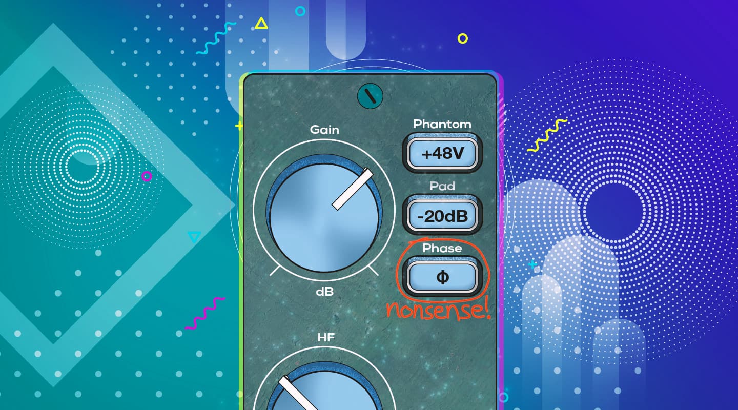
As stated in the previous instalment, pressing the switch on your preamplifier that is incorrectly labelled ‘Phase Reverse’ (or similar nonsense) is not going to fix this problem because, despite its name, that switch does nothing to the signal’s phase; it simply inverts the signal’s polarity. It is applying an amplitude-based solution (polarity inversion) to a time-based problem (phase shift due to delay), and is the wrong tool for the job. As a result of using this switch on one of the two signals, all of the frequencies that were cancelling will now be reinforcing, and all of the frequencies that were reinforcing will now be cancelling. One of those options might sound better than the other, but neither will sound as the musician intended.

PRACTICAL MAGNITUDES
All of the comb filtering examples shown so far – in this instalment and the previous one – are based on worst-case scenarios that assume the original (or ‘direct’) sound and the delayed (or ‘reflected’) sound have been combined at the same magnitudes, resulting in complete cancellation at fc. That’s rarely the case in practice. If the two signals are not combined with the same magnitudes then the cancellations will not be complete nulls and the reinforcements won’t reach the full +6dB – therefore the comb filtering effect is less significant. We’ll explore this practical aspect of comb filtering in the next instalment…

The SI prefixes allow us to turn big numbers with lots of zeroes into small numbers with less zeroes, making them easier to write, read and comprehend. For example, we’re all familiar with k for kilo, which means ‘multiply by 1000’. So 1kg means 1 x 1000 = 1000 grams, 2km means 2 x 1000 = 2000 metres, and 10kHz means 10 x 1000 = 10,000 Hertz. Thanks to the proliferation of computers and mobile devices, we’re also familiar with M for Mega which means ‘multiply by 1,000,000’, G for Giga which means ‘multiply by 1,000,000,000’, and T for Tera which means ‘multiply by 1,000,000,000,000’. If your mobile device has 64GB of memory, it has 64 Gigabytes of memory, or 64 x 1,000,000,000 = 64,000,000,000 bytes of memory.
Similarly, there are SI prefixes for small numbers with lots of zeroes. There is m for milli which means divide by 1000, u for micro which means divide by 1,000,000, n for nano which means divide by 1,000,000,000, and p for pico whch means divide by 1,000,000,000,000.
To understand comb filtering we need to deal with small increments of time, typically measured in thousandths of a second. To simplify those numbers we’ll make use of the SI prefixes m and u, giving us milliseconds (abbreviated to ms and representing thousandths of a second) and microseconds (abbreviated to us and representing millionths of a second). For example, 1ms = 1 millisecond = 1/1000s = 0.001s, and 1us = 1 microsecond = 1/1,000,000s = 0.000001s.
Earlier in this instalment we saw that the frequency of 440Hz has a period of 0.00227 seconds. We can simplify this figure by multiplying it by 1000 to turn it into milliseconds. So, 0.00227s x 1000 = 2.27ms. Conversely, to convert it back to seconds we divide it by 1000, so 2.27ms/1000 = 0.00227s.
ms, m/s and MS confusion
Please be careful not to confuse ms with m/s or MS. It’s important to remember the differences, and understand that ms represents milliseconds and is a measurement of time, m/s represents metres per second and is a measurement of velocity, and MS represents Mid/Side and is a stereo microphone technique and signal processing technique.
Quick Hack
A quick hack to convert seconds (s) into milliseconds (ms) is to move the decimal point three places to the right. To convert milliseconds back into seconds move the decimal point three places to the left. Likewise, to convert seconds (s) into microseconds (us) move the decimal point six places to the right, and to convert microseconds back into seconds move the decimal point six places to the left. So 0.001s becomes 1ms, and 0.000001s becomes 1us. Conversely, 1ms becomes 0.001s, and 1us becomes 0.000001s. Interestingly, a figure such 0.00227 seconds (the period for 440Hz) can be expressed as 2.27ms or 2,270us. In both cases, moving the decimal point the appropriate number of places to the left brings it back to 0.00227 seconds. Check out the tables below for further examples…


RESPONSES