Live Gain Structure

Text: Hugh Covill

THE DECIBEL

When we talk about gain, we can’t avoid talking about the decibel. This measurement is one of the cornerstones of our audio vernacular, but things soon get confusing as there are more dB ‘flavours’ than a Haagen Daaz outlet. There’s dB SPL, dBm, dBv, dBW to dBu, dBV, dB PWL, dBA, dBC and dBVU (and these are just the ones I could think of off the top of my head!). It’s really beyond the scope of this article to define each and every flavour and its associated history, so let’s not get caught in that net just yet. Suffice it to say, the important dB references used in modern sound system gain setting are dBu, dBVU and dBW, and to a much lesser extent dBm and dBV.

The dBm is the original electrical dB reference established in the 1940s, defined as 0dBm = 1 milliwatt @ 600Ω. The 600Ω load related to telephone lines, in that 1mW was the amount of power dissipated when a voltage of 0.775V RMS is applied to a 600Ω telephone line. Most contemporary audio equipment now uses constant voltage interfaces, high-impedance bridging inputs and very low-impedance op-amp outputs. The result is that these devices are not critically load sensitive. As such, dBm is bit of a relic but is worth knowing about, as it makes sense of more modern dB scales.

dBu (the ‘u’ here stands for unterminated) is the current professional audio industry standard reference, and is defined as 0dBu = 0.775 Volts RMS. Note the similarity to the dBm specification. The difference being that dBu is not load sensitive.

dBVU (Volume Unit) is defined as 0dB VU = +4dBu. The VU meter was designed to closely approximate human hearing response, or rather, how we understand volume. It doesn’t track the transient peaks but does a good job of displaying average level (note: it is not an RMS meter, that’s something slightly different again).

dBV is significant only in that most domestic equipment uses this reference and it is not unusual to be asked to connect domestic level gear (iPod’s, MiniDisc players etc.) to a PA. Domestic gear output level is –10dBV (approximately 1/3 of a volt). 0dBV = 1Volt RMS.

dBW is defined as 0dBW = 1 Watt. A 500W power amp can be thought of as a 27dBW amp. (See Fig. #2)

To properly set sound system gain structure we also need to understand RMS level and Peak level. RMS (Root Mean Square), put simply, is a mathematical formula that expresses the power inherent in a complex waveform (think of it as the area of the waveform). We can consider it as the average level (although that’s not empirically true). Peak level is the maximum level possible before clipping, i.e., the maximum signal voltage that a circuit can provide before it square waves.

DYNAMIC RANGE & HEADROOM

Dynamic range, expressed in decibels, is the ratio (comparison) of the peak signal level possible compared to the noise floor. The maximum output level will generally be in the +18dBu to +28dBu range. The best noise floor numbers are around 85–90dBu. So, dynamic range figures in the order of >110dB are not uncommon on spec sheets.

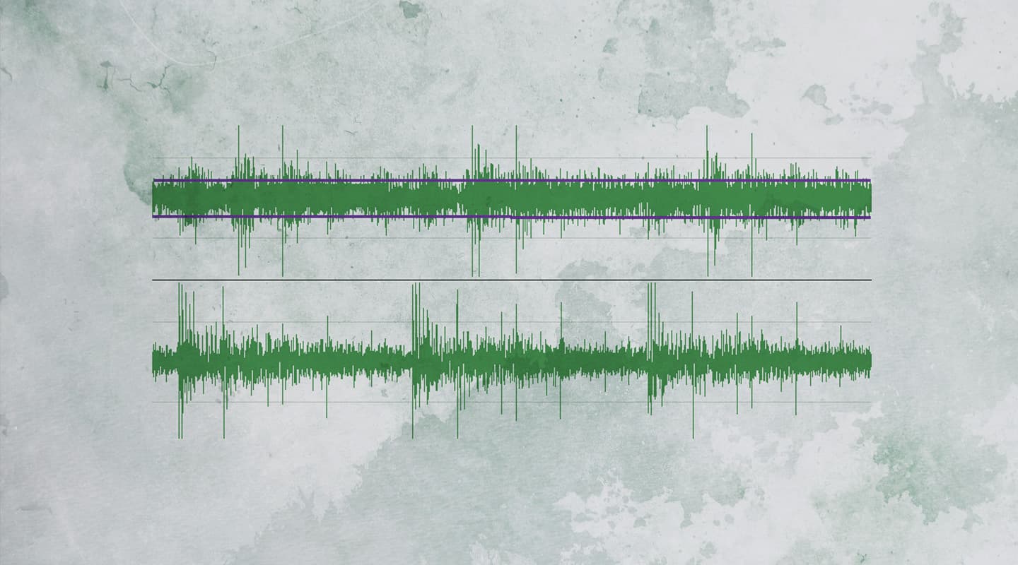
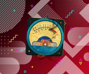
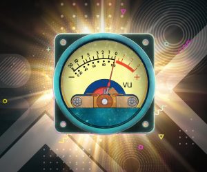
‘Headroom’ describes a device or system’s ability to handle transient peaks in the program. It’s also expressed in decibels and is the ratio of the maximum output level to that of the nominal operating signal level. Consider Fig. #3 for a moment. It’s a picture of a waveform. The difference between the average level and the peaks is how much headroom will be required to reproduce that waveform.

Examining Fig.1 we see our nominal operating level is +4dBu = 0dBVU (1.23 Volts) and the largest level before clipping is +26dBu, (15.5 Volts), thus we have 22dB of headroom.

The important thing to grasp with sound reinforcement systems is that the noise floor is actually defined by the background noise of the venue (acoustical noise floor). This will involve factors such as loud audience noise, background air-conditioning noise and even moving light noise. Acoustically, the maximum output level will be the loudest SPL the system needs to produce. When using microphones it may be determined by the gain before feedback and the feedback stability margin you wish to use. If we compare (ratio) the loudest SPL (say 105dB SPL) to the background noise (which may be in the range of 30 to 55dB SPL) it becomes clear that useable dynamic range in a sound reinforcement system is a far cry from the individual component specifications (perhaps as little as 50dB). Options are limited. We need to mix at a sound pressure level that is appropriate for the style of music. Turning up the volume may not only be artistically untenable but can also represent a safety risk for the audience in terms of exposure to overly high sound volumes. (It is also extremely important to protect venue staff that may be exposed to high SPL levels night after night on a long-term basis.) Consequently the dynamic range of a sound reinforcement system is defined by factors (largely) beyond our control. What we can control is system headroom. The amount of headroom required will depend on the program material. For classical music it may be 30dB; for rock music that utilises a lot of dynamics processing, as little as 10dB may be enough. As a rule of thumb, 20dB is a good number to aim for. So here are two methods of optimising headroom.

OPTIMISING HEADROOM

Unity Method – Our first approach is often called the ‘Unity’ method because it involves setting a unity gain output at the console and all subsequent processing through to the amps. The idea being that the unity gain (no increase or decrease in signal level) output from the console will be what the amp sees at input after it has passed through all the system electronics. This method is quick and easy and is preferred in situations where you have limited time; where you can’t use test equipment; where the system is reconfigured regularly; and where you’re often introducing hired gear of uncertain specifications. It will provide a consistent level through the system but you also expose yourself to the possibility of clipping devices downstream, as well as reducing the signal-to-noise ratio. This is probably the most commonly utilised method.

Clip Together – For critical listening applications where you have the time to build a sound system for a particular application, the preferred method is to adjust each system component to hit clip simultaneously with the mixing desk. The advantages are that the mixing desk meters become the system meters and you maximise dynamic range through each component. It is not suitable for a system that is re-patched regularly as the level will be inconsistent through the system.

Whichever method you choose to set the system gain, do it with any equalisation or compression bypassed and the amps powered down. The amplifiers should be the last component optimised. So for gain setting a system where all devices clip simultaneously you need to generate a test signal at an input to the mixer. Adjust the gain until the input clip indicator lights up and then back off a little. (Pink noise is a good choice of test signal as it best represents the broad spectral content of music program.) Now generate the maximum output level possible from the main outs. If the next component has input and output gain trims and meters, set them to momentarily light the clip indicators. If there’s only one gain trim, use that in the same fashion. Fig.4 demonstrates a system with 16dBu of headroom and all components hitting clip together.

SETTING THE AMPLIFIER

Setting the appropriate amplifier level is a much-misunderstood art (I’m presupposing that the speakers and amps are suitably matched, which is an article in its own right). The most important concept to grasp is that professional amp control knobs do not relate to volume or power. They are input attenuators. The input sensitivity number tells us that, with the input attenuator control set to zero (full), the amp will be delivering its full output power. Voltage anywhere beyond this is clipping the amplifier.

Take a look at Fig. 5 (a fairly standard amplifier control knob). This knob acts in just the same way as your pad switch does on a console. If a signal were overloading the input to your console you would pad it down. Similarly, your amplifier’s knob is there to pad down signals that are going to clip the amp.

Amplifiers seem to have no input sensitivity standard so you will see specifications range from 0.775V RMS through to 1.5V RMS (0dBu through to +6dBu). If we examine Fig. 4 again we can see that our DSP unit is outputting +4dBu but our amplifier only requires 0dBu to produce full power, thus we need to attenuate 4dB to give our amp 0dBu then add our 16dB of headroom. We attenuate the input to the amp by 20dB (yes, turn it down) to have the amp producing its full power potential while maintaining headroom.

GAINING SOME INSIGHT

Presented in this article are the fundamental concepts that underpin setting system gain for live sound reinforcement, and inevitably I’ve skated over many elements in pursuit of the bigger picture. Gain structure through the console, amp settings for providing power to specific pass bands (bi-amping etc), the use of system-wide compressor/limiters and digital system gain architecture are subjects in there own right, which we’ll pursue in coming issues of AT. This article is a primer to encourage us all to investigate our own gain structure techniques further. The diagrams present simplistic system schematics but the concepts they demonstrate will hold for the most complex PA systems. There are other methodologies that you’ll see in the field and many employ certain compromises for the sake of system simplicity. However, the base concepts remain constant and a strong grasp of these makes understanding other topologies and their rationale simple. Turning amps up to full without regard to input sensitivity is a deeply flawed practice. Often a harsh sound system can be traced to amps clipping (don’t even get me started on amplifying the electrical noise floor!).

If your gain structure is correct through the entire system, and you can’t reach your desired SPL, it’s time to add more speakers. Incorrect gain structure is one of the foremost reasons for bad live sound. Proper settings can markedly improve any live sound system.